


Conditional Formatting
Across the whole row!
Introduction
 Conditional formatting is a great way to use colour and other features to make particular results in a table stand out. Conditionally formatting cells in a single column is easy to do. It is often more useful, however, if we can conditionally format an entire row of cells in a table based upon the condition in a single column. Setting this up is actually quite easy but is not the most obvious in how to do it.
These notes are for Google Sheets however the concpets discussed here will work in a similar manner within MS Excel as well.
The screenshots and instructions here are for Google Sheets at the time this page was created. Google regularly updates its products and interface layout so you may encounter a slightly different looking interface. Everything should still function the same however.
First off, what is conditional formatting?
Conditional formatting allows us to change the formatting of cells based upon certain criteria. This is a valuable feature as humans are visual by nature and it allows us to make certain data really stand out.
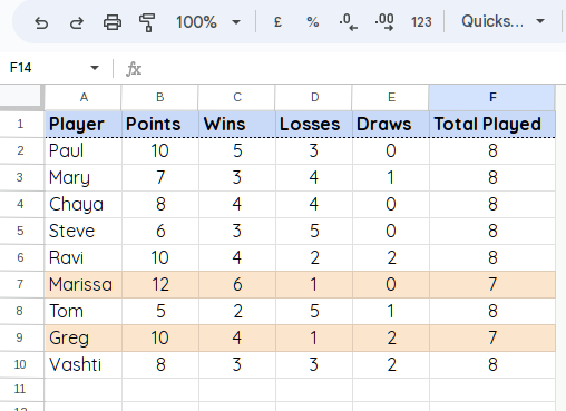
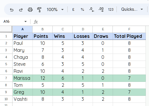
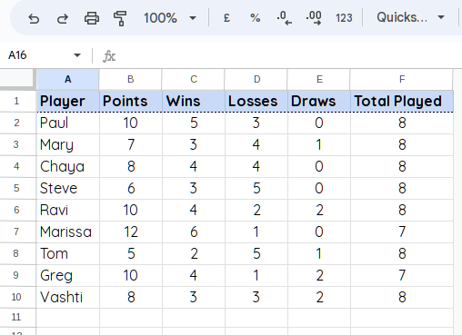 Let's say that we have the following table of data to the right. Players need to play a total of 8 games each but we haven't finished the competition yet. We can see that that is the case by scanning down the Total Played column. It would be nicer, though, if players with games still to play were made clearer.
Highlight the target data
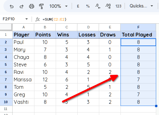 First off, we select the data that we wish to apply the conditional formatting to. In this case it is cells F2 - F10.
Open up Conditional Formatting
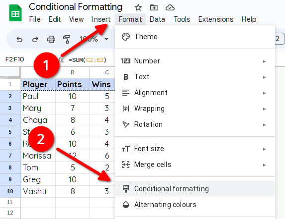 Next we need to open up the Conditional Formatting side panel.
Set the condition
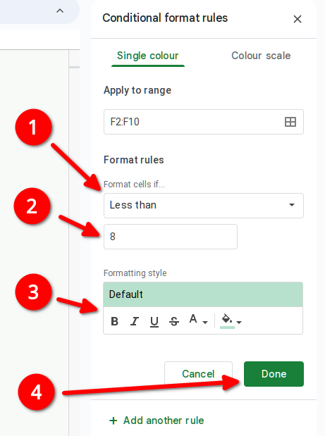 Next we will change the format rule.
The rule will be Less than and we will set the value to 8.
Change the formatting style to better suit your needs.
Then click Done and your rule is set.
The result
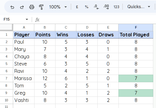 And now we can more easily see which players still have games to play.
You can always re open the Conditional Formatting panel and change the formatting style at any point if you want to change the formatting style or any other parameters.
This was simple to achieve but it still requires a bit of work for the viewer. To konw which players are still needing to play we need to scan across to column A but there is effort involved in making sure we line up with the required cells from column F. Wouldn't it be much better if the whole row was highlighted instead for the relevant entries?
Conditionally Formatting an Entire Row
Now let's perform the same activity but make the whole rows stand out.
Highlight the target data
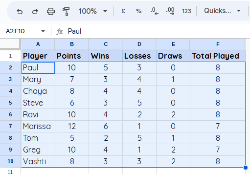 This time we will select the whole table of data from A2 - F10.
Open up Conditional Formatting
Next we need to open up the Conditional Formatting side panel. (same as before)
Set the condition
 Next we will change the format rule.
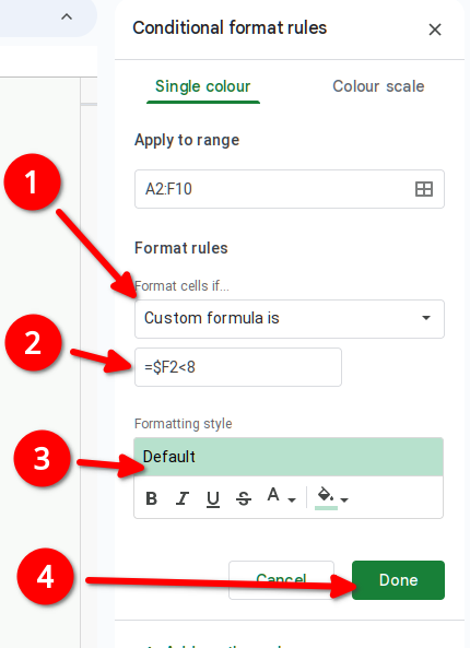
This time we will scroll down to the bottom of the Format cells if menu and select Custom Formula is
The formula will be = $F2 < 8
The dollar sign ( $ ) in front of F indicates that this is an absolute reference rather than the usual relative reference. If you remove the $ sign you will notice that almost all the cells get formatted. This is because as you move across into cells in columns B, C, D etc it will start comparing to values in columns G, H, I etc (which don't exist here and hence have a logical value of 0).
Change the formatting style to better suit your needs.
Then click Done and your rule is set.
The result
 And now we can more easily see which players still have games to play.
You can always re open the Conditional Formatting panel and change the formatting style at any point if you want to change the formatting style or any other parameters.
Another Example
Let's also highlight the winning player (that with the highest score). What you will notice is that the player with the highest score is Marissa, who is already having formatting applied due to not already having played 8 games. This will allow us to illustrate how the ordering of several rules is important in how they are applied.
 Run through the same steps as before however when entering the panel you will see that the rule we made previously is there and an option to Add another rule which is what we will do.
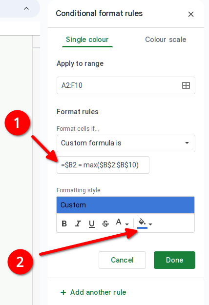
Set up as before however when entering the formula, insert the following formula instead :
= $B2 = max($B$2:$B$10)
We will also set the background colour to be Blue so that the winning player stands out from those that need to play more games.
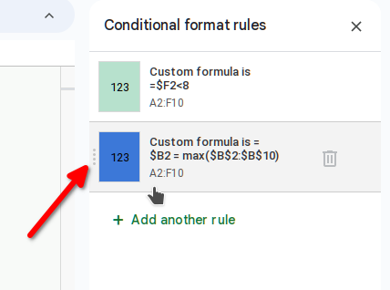 When you select Done you will notice that nothing appears to happen. This is because the new rule is listed below the first one. Once a rule has been applied to a cell, no further rules will be applied to it. To fix this up and get the behaviour we desire we need to reorder the rules. When you hover your mouse over a rule you will notice four dots appear to the left of the rule. Clicking on this, you may drag the rule to reorder them. When we do this you should notice that Marissa now gets formatted as the winning player.
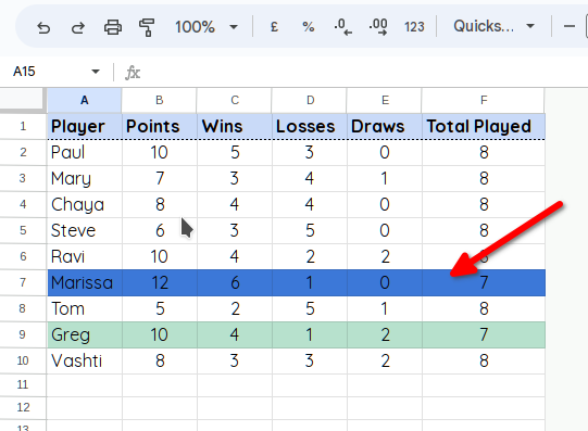 And now we have our combined conditional formatting.
The screenshots and instructions here are for Google Sheets at the time this page was created. Google regularly updates its products and interface layout so you may encounter a slightly different looking interface. Everything should still function the same however.


